Game Math: Curve Approximation via Curve “Projection”

This post is part of my Game Math Series.

Also, this post is part 2 of a series (part 1) leading up to a geometric interpretation of Fourier transform and spherical harmonics.

Drawing analogy from vector projection, we have seen what it means to “project” a curve onto another in the previous post. This time, we’ll see how to find a the closest vector on a plane via vector projection, and then we’ll see how it translates to finding the best approximation of a curve via curve “projection”. This handy analogy can help us take another step closer to a geometric interpretation of Fourier transform and spherical harmonics later.

Closest Vector on a Plane

Given vectors $\vec{a}$ , $\vec{b}$ , and $\vec{c}$ , the closest vector on the plane formed (or “spanned” in linear algebra jargon) by $\vec{b}$ and $\vec{c}$ is the projection of $\vec{a}$ onto the plane. This projection, denoted $\vec{d}$ , is a combination of scaled $\vec{b}$ and $\vec{c}$ , in the form of $\vec{d} = u \vec{b} + v \vec{c}$ , that has the least error from $\vec{a}$ .

The error is measured by the magnitude of the difference vector:

$err(\vec{a}, \vec{d}) = |\vec{a} - \vec{d}| \\$

As pointed out in the previous post, minimizing this error is essentially equivalent to minimizing the root mean square error (RMSE):

$\text{minimize} \enspace err(\vec{a}, \vec{d}) \enspace \Leftrightarrow \enspace \text{minimize} \enspace RMSE(\vec{a}, \vec{d})$

This is what the relationship of $\vec{a}$ , $\vec{b}$ , $\vec{c}$ , and $\vec{d}$ looks like visually:

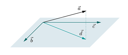
The projection of $\vec{a}$ onto the plane spanned by $\vec{b}$ and $\vec{c}$ , is the vector $\vec{d}$ on the plan that has the least error from $\vec{a}$ , and the difference vector $\vec{a} - \vec{d}$ is orthogonal to the plane.

So how do we compute $\vec{d}$ ? In the previous post we’ve seen how to project a vector onto another, so would computing $\vec{d}$ be as simple as projecting $\vec{a}$ onto $\vec{b}$ , and then project the result again onto $\vec{c}$ ? Not really. Here’s why:

As you can see in the figure above, $\vec{d}$ isn’t parallel to $\vec{b}$ nor $\vec{c}$ . Projecting $\vec{a}$ onto $\vec{b}$ would give you a vector that is parallel to $\vec{b}$ , and a subsequent projection onto $\vec{c}$ would leave you with a result that is parallel to $\vec{c}$ , which is definitely not $\vec{d}$ .

One way to do it is to calculate a vector orthogonal to the plane, i.e. a plane normal $\vec{n}$ , by taking the cross product of the two vectors that span the plane: $\vec{n} = \vec{b} \times \vec{c}$ . Then, take out the part in $\vec{a}$ that is parallel to $\vec{n}$ by subtracting the projection of $\vec{a}$ onto $\vec{n}$ from $\vec{a}$ . What is left of $\vec{a}$ is the part of $\vec{a}$ that is parallel to the plane, i.e. the projection:

$\begin{flalign*} \vec{n} &= \vec{b} \times \vec{c} \\ \vec{d} &= \vec{a} - proj(\vec{a}, \vec{n}) \\ \end{flalign*}$

But, I want to talk about another way of performing the projection, which is easier to translate to curves later. $\vec{b}$ and $\vec{c}$ are not necessarily orthogonal to each other. Let’s find two orthogonal vectors that lie on the plane spanned by $\vec{b}$ and $\vec{c}$ . Then, we split $\vec{a}$ into two parts, one parallel to one vector and one parallel to the other vector. Finally, we combine these two parts together to obtain a vector that is essentially the part of $\vec{a}$ that is parallel to the plane.

As a simple illustration, if the plane is the X-Z plane, then the obvious two orthogonal vectors of choice would be $(1, 0, 0)$ and $(0, 0, 1)$ . To project a vector $(4, 5, 6)$ onto the X-Z plane, we split it into a part that is parallel to $(1, 0, 0)$ , which is $(4, 0, 0)$ , and a part that is parallel to $(0, 0, 1)$ , which is $(0, 0, 6)$ . Combining those two parts together would give us $(4, 0, 6)$ . This makes sense, because projecting a vector onto the X-Z plane is just as simple as dropping the Y component.

Now, given two arbitrary vectors $\vec{b}$ and $\vec{c}$ that span a plane, we can generate two orthogonal vectors, denoted $\vec{e}_0$ and $\vec{e}_1$ , by using a method called the Gram-Schmidt process. The first vector $\vec{e}_0$ would simply be the $\vec{b}$ . To compute the second vector $\vec{e}_2$ , we take away from $\vec{c}$ its part that is parallel to $\vec{b}$ ; what’s left of $\vec{c}$ is orthogonal to $\vec{b}$ :

$\begin{flalign*} \vec{e}_0 &= \vec{b} \\ \vec{e}_1 &= \vec{c} - proj(\vec{c}, \vec{e}_0) \\ \end{flalign*}$

To compute $\vec{d}$ , we combine the parts of $\vec{a}$ that are parallel to $\vec{e}_0$ and $\vec{e}_1$ , respectively:

$\begin{flalign*} \vec{a}_0 &= proj(\vec{a}, \vec{e}_0) \\ \vec{a}_1 &= proj(\vec{a}, \vec{e}_1) \\ \vec{d} &= \vec{a}_0 + \vec{a}_1 \end{flalign*}$

More on Gram-Schmidt Process

The Gram-Schmidt process is actually more general than described above. It can apply to higher dimensions. Given $M$ vectors, denoted $\vec{p}_0$ to $\vec{p}_{M-1}$ , in an $N$ -dimensional space ( $N > M$ ), and if the $M$ vectors are linearly independent, i.e. they span an $M$ -dimensional subspace, then we can generate $M$ vectors that are orthogonal to each other, denoted $\vec{q}_0$ through $\vec{q}_{M-1}$ , spanning the same subspace, using the Gram-Schmidt process.

The first vector $\vec{q}_0$ would simply be $\vec{p}_0$ . To compute the second vector $\vec{q}_1$ , we take away from $\vec{p}_1$ its part that is parallel to $\vec{p}_0$ . To compute the third vector $\vec{q}_2$ , we take away from $\vec{p}_2$ its part that is parallel to all previously generated orthogonal vectors, $\vec{p}_0$ and $\vec{p}_1$ . Repeat this process until we have reached $\vec{p}_{M-1}$ and produced $\vec{q}_{M-1}$ :

$\begin{flalign*} \vec{q}_0 &= \vec{p}_0 \\ \vec{q}_1 &= \vec{p}_1 - proj(\vec{p}_1, \vec{q}_0) \\ \vec{q}_2 &= \vec{p}_2 - proj(\vec{p}_2, \vec{q}_0) - proj(\vec{p}_2, \vec{q}_1) \\ ... \\ \vec{q}_{M-1} &= \vec{p}_{M-1} - \sum^{M-2}_{i=0}{proj(\vec{p}_{M-1}, \vec{q}_i)} \\ \end{flalign*}$

Projecting an $N$ -dimensional vector onto this $M$ -dimensional subspace would involve combining the parts of the vector parallel to each of the orthogonal vectors. In our example above that involves 3D vectors, $M = 2$ and $N = 3$ . In higher dimensions, no simple 3D cross products can save you there.

Now we are done with vectors. Let’s take a look at curves!

Curve Approximation

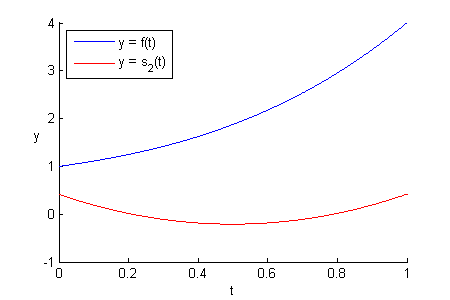
Let’s say our interval of interest is $0 \leq t \leq 1$ . Given a 3rd-order polynomial curve $f(t) = 1 + t - t^2 + t^3$ , what’s the best approximation using a 2st-order polynomial curve, or a 1th-order polynomial curve (flat line)? How about simply dropping the higher-order terms, so we get $f_2(t) = 1 + t - t^2$ and $f_1(t) = 1 + t$ ? Here’s what they look like:

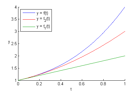
At first glance, I’d say $f_2(t)$ and $f_1(t)$ are not what we want. We can definitely find a parabolic curve and a line that approximate $f(t)$ better. Look at just how far apart $f_2(t)$ and $f_1(t)$ are from $f(t)$ at $t = 1$ . Clearly, $f_2(t)$ and $f_1(t)$ are not the 2nd-order and 1st-order polynomial curves that have the least RMSEs from $f(t)$ . Simply dropping higher-order terms turns out to be a naive approach. The right way to do it is just like what we did with vectors: projection.

In the vector example above, we were operating in the 3D geometric space. Now we are working with a more abstract 3rd-order polynomial space where $f(t)$ lives in. The lower-order polynomial curve that has the least RMSE from $f(t)$ is the projection of $f(t)$ into that lower-order polynomial space. Let’s start with finding the 2nd-order polynomial curve that has the least RMSE from $f(t)$ .

The 2nd-order polynomial subspace is 3-dimensional, since a 2nd-order polynomial curve has the form $x + y t + z t^2$ . Let’s first find 3 curves that span the subspace. An easy pick would be $j_0(t) = 1$ , $j_1(t) = t$ , and $j_2(t) = t^2$ . Now we need to use them to generate a set of orthogonal curves, $k_0(t)$ , $k_1(t)$ , and $k_2(t)$ using the Gram-Schmidt process:

$\begin{flalign*} k_0(t) &= j_0(t) \\ k_1(t) &= j_1(t) - proj(j_1(t), k_0(t)) \\ k_2(t) &= j_2(t) - proj(j_2(t), k_0(t)) - proj(j_2(t), k_1(t)) \\ \end{flalign*}$

If you forgot how to “project” a curve onto another, please refer to the previous post.

Here are the results:

$\begin{flalign*} k_0(t) &= 1 \\ k_1(t) &= \dfrac{-1}{2} + t \\ k_2(t) &= \dfrac{1}{6} - t + t^2 \\ \end{flalign*}$

You can say that $k_0(t)$ , $k_1(t)$ , and $k_2(t)$ are a set of orthogonal axes spanning the 2nd-order polynomial subspace. Now we split $f(t)$ into three orthogonal parts by projecting it onto $k_0(t)$ , $k_1(t)$ , and $k_2(t)$ :

$\begin{flalign*} s_0(t) &= proj(f(t), k_0(t)) = \dfrac{25}{12} \\ s_1(t) &= proj(f(t), k_1(t)) = \dfrac{-29}{10} + \dfrac{29}{20}t \\ s_2(t) &= proj(f(t), k_2(t)) = \dfrac{5}{12} - \dfrac{-5}{2}t + \dfrac{5}{2}t^2 \\ \end{flalign*}$

Here’s what $s_0(t)$ , $s_1(t)$ , and $s_2(t)$ look like alongside $f(t)$ :

$s_1(t)$ and $s_2(t)$ might not look like they are close to $f(t)$ , but they are the closest curves you can get along the axes $k_1(t)$ and $k_2(t)$ that have the least RMSEs from $f(t)$ .

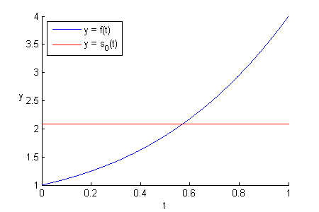
Now, we can combine the three orthogonal parts of $f(t)$ to form the 2nd-order polynomial curve that is the best approximation of $f(t)$ :

$\begin{flalign*} g(t) &= s_0(t) + s_1(t) + s_2(t) \\ &= \dfrac{21}{20} + \dfrac{2}{5}t + \dfrac{5}{2}t^2 \\ \end{flalign*}$

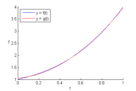
This looks way better than the result of simply dropping the 3rd-order term, as shown in the figure above.

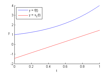
Since the three parts are already orthogonal, we can actually obtain the 1st-order polynomial curve that best approximates $f(t)$ by simply dropping $s_2(t)$ from $g(t)$ :

$\begin{flalign*} h(t) &= s_0(t) + s_1(t) \\ &= \dfrac{19}{30} + \dfrac{29}{10}t \\ \end{flalign*}$

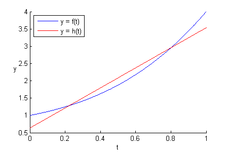
Also looking good, compared to simply dropping the 3rd-order and 2nd-order terms.

That’s it. In this post, we’ve seen how to generate a set of orthogonal curves from a set of curves spanning a lower-dimensional subspace of curves, and use the orthogonal curves to find the best approximation of a curve via curve “projection”.

We now have all the tools we need to move onto Fourier transform and spherical harmonics in the next post. Finally, something game-related!

3 Responses to Game Math: Curve Approximation via Curve “Projection”

Kamil says:

March 23, 2017 at 03:08

This is really great! 🙂 When we could expect the next part? I’m not trying to hurry you, I can imagine that writing on such topic is not an easy task (or at least not a quick task). I’m just wondering if you already scheduled the next part? Or is it postpone when you have more time?

- Allen Chou says:
  
  March 23, 2017 at 07:24
  
  It’s on my list. But there are other things going on right now, so it’s currently not my top priority.
  
  - Kamil says:
    
    March 23, 2017 at 07:28
    
    I see. Thanks for the quick answer.

Closest Vector on a Plane

More on Gram-Schmidt Process

Curve Approximation

Related

About Allen Chou

3 Responses to Game Math: Curve Approximation via Curve “Projection”

Leave a ReplyCancel reply

Search

Follow Me

Categories

Archives

Meta

Feeds

Game Math: Curve Approximation via Curve “Projection”

Closest Vector on a Plane

More on Gram-Schmidt Process

Curve Approximation

Share this:

Related

About Allen Chou

3 Responses to Game Math: Curve Approximation via Curve “Projection”

Leave a ReplyCancel reply

Search

Follow Me

Categories

Archives

Meta

Feeds