
This post is part of my Game Math Series.
While processing data for skeletal animations, we are usually faced with a series of discrete samples of positions and orientations. The positional samples are typically stored as a series of 3D vectors, and the orientational samples are typically stored as a series of quaternions. The most straightforward way to interpolate between positional samples is using piece-wise lerp (linear interpolation), and the counterpart for orientational samples is using piece-wise slerp (spherical linear interpolation). For more information on slerp, please see my previous post on quaternion basics.
The samples are sometimes too far apart, and we can see the visual artifact of discontinuous change in the first-order derivative of interpolation, i.e. the interpolation is not smooth at sample points.
In this post, I will present to you a technique for interpolating orientational samples in a smooth fashion called circular blending. I leaned about this technique from the MAT 351 class at DigiPen, taught by professor Matthew Klassen.
Let’s say we are given a series of quaternions:
![\[ q_0, q_1, q_2, ..., q_n \]](https://allenchou.net/wp-content/ql-cache/quicklatex.com-9383fc1b85b43b6d30f2570418e4d4b0_l3.png "Rendered by QuickLaTeX.com")
Let  and
and  denote the two quaternions we are trying to interpolate between, and let
  denote the interpolation parameter (
 ). Also, let
  denote the interpolating curve between and .
If we are just using the straightforward slerp approach, we get:
![\[ r_i(t) = Slerp(q_i, q_{i + 1}, t) \]](https://allenchou.net/wp-content/ql-cache/quicklatex.com-5f7073c8f74df33fc311442bdb828218_l3.png "Rendered by QuickLaTeX.com")
This is a  curve, meaning the curve is only continuous up to the zeroth-order derivative, i.e. the curve itself. The first-order derivative is generally not continuous at sample points using this approach.
Circular blending gives us a nice  curve, which means the curve is continuous up to the first-order derivative. It is difficult to visualize quaternions, so I will use a 2D analogy to explain how circular blending works and how to mathematically work it out.
Theory
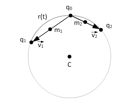
In order to interpolate between two quaternions and using circular blending, we also need the two neighboring samples  and
and  . Let the figure below represent the four sample points:

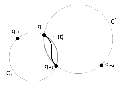
If we just use piece-wise slerp, this is what the curve will look like:

We can easily see the abrupt change of slope at sample points.
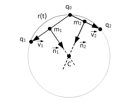
To prepare for circular blending between and , we draw two circles; one passes through  , , and ; the other one passes through , , and . Let us denote these two circles
  and
and  , respectively. Also, let us denote the arcs on these circles going from to as
  and
and  , with
  and
and  .
.
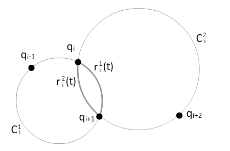
The formula for circular blending between and is as follows:
![\[ r_i(t) = Slerp(r^1_i(t), r^2_i(t), t) \]](https://allenchou.net/wp-content/ql-cache/quicklatex.com-41dd9f96441177f0ec89755590e8ddaf_l3.png "Rendered by QuickLaTeX.com")
It is as simple as taking the slerp between the two arcs connecting and . The arc fully contributes to the slope at , and the arc fully contributes to the slope at .
So why does this give us a curve? Let’s add the curve between the next pair of samples, and . We need another sample  in order to draw the circle
  .
.
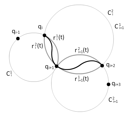
Notice how the arc  fully contributes to the slope of
  at . The arc is part of the same circle as the arc
  , so the slope is continuous at the sample point .
Now let’s look at how we can find these circles and the desired arcs.
Details & Derivation
Given three points,  ,
,  , and
, and  , we would like to find a circle that passes through these points. Let
  denote the center of this circle. Also, we would like to find the parameterized arc
  that goes from to , where
  and
and  .
.
Let  denote the vector from to , and let
  denote the vector from to . Let
  denote the midpoint between and , and let
  denote the midpoint between and .
If we draw the bisectors of and , they should pass through the center of the circle, because a bisector of a line segment connecting two points on a circle always passes through the center of the circle. The bisectors are perpendicular to their corresponding vectors and . Let the direction vectors of the two bisectors be denoted as  and
and  .
.
To find and , we use the formulas:
![\[ \overrightarrow{n_1} = \overrightarrow{v_2} - proj_{\overrightarrow{v_1}}(\overrightarrow{v_2}) \]](https://allenchou.net/wp-content/ql-cache/quicklatex.com-2e62c51c7f27a459ce9297b4970305f8_l3.png "Rendered by QuickLaTeX.com")
![\[ \overrightarrow{n_2} = \overrightarrow{v_1} - proj_{\overrightarrow{v_2}}(\overrightarrow{v_1}) \]](https://allenchou.net/wp-content/ql-cache/quicklatex.com-6a10148e1682136e0273b1e29647f634_l3.png "Rendered by QuickLaTeX.com")
where  denotes the projection of the vector
  onto the vector
  .
.
Now we have the parameterized formula for the two bisectors,  and
and  :
:
![\[ b_1(s) = m_1 + s \overrightarrow{n_1} \]](https://allenchou.net/wp-content/ql-cache/quicklatex.com-9aadc5c659b29209a270cc7e15f505c7_l3.png "Rendered by QuickLaTeX.com")
![\[ b_2(t) = m_2 + t \overrightarrow{n_2} \]](https://allenchou.net/wp-content/ql-cache/quicklatex.com-ac0f8e30a725dbb19f3301b086724121_l3.png "Rendered by QuickLaTeX.com")
The center of the circle is at the intersection of these two bisectors, so we need to find the parameter pair  that satisfies:
![\[ m_1 + s \overrightarrow{n_1} = m_2 + t \overrightarrow{n_2} \]](https://allenchou.net/wp-content/ql-cache/quicklatex.com-40cc10dcb89fba393a91fd27a08e339d_l3.png "Rendered by QuickLaTeX.com")
If we rearrange the equation, we get:
![\[ s \overrightarrow{n_1} - t \overrightarrow{n_2} = m_2 - m_1 \]](https://allenchou.net/wp-content/ql-cache/quicklatex.com-f8361eec8cfcebd74ab79d6930b9aee3_l3.png "Rendered by QuickLaTeX.com")
Remember that we are working with quaternions, so the vectors , , and  are all 4D vectors. This means that we have four equations for two unknowns, which is more than enough. All we have to do is to pick two equations and use Cramer’s Rule to solve for . Beware that the two equations you choose might not have a solution, i.e. you get a zero determinant when applying Cramer’s Rule; so be sure pick two equations that do not give you a zero determinant when solving for . We can obtain by plugging either
  or back into its corresponding bisector equation.
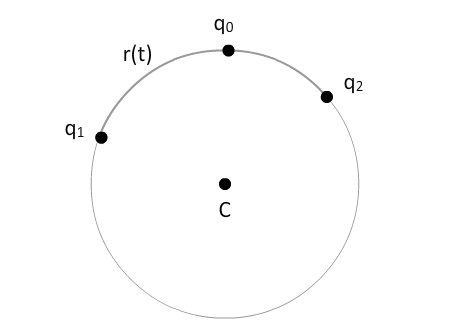
Now that we have the center of the circle , the last step is to find the parameterized arc where and . We aim to find the arc in the following form:
![\[ r(t) = C + R(cos(t\theta)\overrightarrow{u} + sin(t\theta)\overrightarrow{v}), \]](https://allenchou.net/wp-content/ql-cache/quicklatex.com-9438d6ba72849396db38764fd4a7a80d_l3.png "Rendered by QuickLaTeX.com")
where  is the angle between and , so
  ;
;  is the radius of the circle;
  and
and  form an orthonormal basis of the plane that contains the circle.
Finding is easy. It is the unit vector pointing from to :
![\[ \overrightarrow{u} = \frac{q_1 - C}{|q_1 - C|} \]](https://allenchou.net/wp-content/ql-cache/quicklatex.com-ebe70a8db21e5448915599bcb0e0e09c_l3.png "Rendered by QuickLaTeX.com")
As for finding , we first find the unit vector  pointing from to :
![\[ \overrightarrow{w} = \frac{q_2 - C}{|q_2 - C|} \]](https://allenchou.net/wp-content/ql-cache/quicklatex.com-5085c4f2c68f847243d788276f00cc2f_l3.png "Rendered by QuickLaTeX.com")
and then we can find by taking out from its parallel component to :
![\[ \overrightarrow{v} = \frac{\overrightarrow{w} - proj_{\overrightarrow{u}}(\overrightarrow{w})}{|\overrightarrow{w} - proj_{\overrightarrow{u}}(\overrightarrow{w})|} \]](https://allenchou.net/wp-content/ql-cache/quicklatex.com-058b0cc502295894f6fefb213d592c92_l3.png "Rendered by QuickLaTeX.com")
Visually, here’s the whole picture:
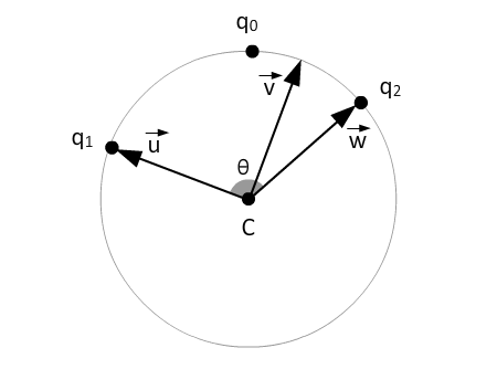
We are done! We have found the circle that passes through the three points, as well as the parameterized arc on the circle that satisfies and .
One last thing. You might wonder what we should do if the three points are collinear. There’s no way we can find a circle with finite radius that passes through three collinear points! Remember that we are working with unit quaternions here. Three different unit quaternions would never be collinear because they lie on three different spots on the 4D unit hypersphere, just as three different points on a 3D unit sphere would never be collinear. So we are good.
Demo
Finally, let’s look at a video comparing the results of piece-wise slerp and circular blending in action.

Interesting idea, but why not simply use Catmull-Rom splines? The math is simpler, plus game engines will likely have spline interpolation code already. One could even consider Hermite splines with user-controlled tangents, as is usually done for other animation curves, though I’m not sure how useful this would really be with quaternion.
Yes, the math for Catmull-Rom splines is indeed simpler. I hope I’m not giving the wrong impression that circular blending is superior than any other interpolation techniques; I just wanted to present one of the techniques that can be used to smoothly interpolate quaternions.