
This post is part of my Game Math Series.
Source files are on GitHub
Previously, I talked about numeric springing and provided some examples.
I have been saving up miscellaneous topics I would like to discuss about numeric springing, and now I have enough to write another post. Here are the topics:
- Using The Semi-Implicit Euler Method
- Numeric Springing vs. Tweening
- Half-Life Parameterization
Using The Semi-Implicit Euler Method
Recall the differential equation for a damped spring:
![\[ \frac{\mathrm{d}^2 x}{\mathrm{d} t^2}} + 2 \zeta \omega \frac{\mathrm{d} x}{\mathrm{d} t}} + \omega^2 (x - x_t) = 0 \]](http://allenchou.net/wp-content/ql-cache/quicklatex.com-718f51c540bea215dcd95035ab866442_l3.png "Rendered by QuickLaTeX.com")
And the equations for simulating such system obtained by the implicit Euler method:

where:

I presented the equations obtained by the implicit Euler method, because they are always stable. We can obtain a different set of equations that can also be used to simulate a damped spring system by the semi-implicit Euler method:

The equations obtained by the semi-implicit Euler method involve much less arithmetic operations, compared to the equations obtained by the implicit Euler method. There is a catch: the equations obtained by the semi-implicit Euler method can be unstable under certain configurations and the simulation will blow up over time. This can happen when you have a large  and
and  . However, the and on most use cases are far from the breaking values. You would almost never use an overdamped spring, so is usually kept under 1. Even if is set to 1 (critically damped spring), can be safely set up to
  (5Hz), which is a very fast oscillation you probably would never use on anything.
So, if your choice of and result in a stable simulation with the equations obtained by the semi-implicit Euler method, you can use them instead of the equations obtained by the implicit Euler method, making your simulation more efficient.
Here’s a sample implementation:
/*
  x     - value             (input/output)
  v     - velocity          (input/output)
  xt    - target value      (input)
  zeta  - damping ratio     (input)
  omega - angular frequency (input)
  h     - time step         (input)
*/
void SpringSemiImplicitEuler
(
  float &x, float &v, float xt,
  float zeta, float omega, float h
)
{
  v += -2.0f * h * zeta * omega * v
       + h * omega * omega * (xt - x);
  x += h * v;
}
Numeric Springing vs. Tweening
Numeric springing and tweening (usually used with the famous Robert Penner’s easing equations) might seem very similar at first, as they are both techniques to procedurally animate a numeric value towards a target value; however, they are actually fundamentally different. Tweening requires a pre-determined duration; numeric springing, on the other hand, does not have such requirement: numeric springing provides a simulation that goes on indefinitely. If you were to interrupt a procedural numeric animation and give it a new target value, numeric springing would handle this gracefully and the animation would still look very natural and smooth; it is a non-trivial task to interrupt a tweened animation, set up a new tween animation towards the new target value, and prevent the animation from looking visually jarring.
Don’t get me wrong. I’m not saying numeric springing is absolutely superior over tweening. They both have their uses. If your target value can change dynamically and you still want your animation to look nice, use numeric springing. If your animation has a fixed duration with no interruption, then tweening seems to be a better choice; in addition, there are a lot of different easing equations you can choose from that look visually interesting and don’t necessarily have a springy feel (e.g. sine, circ, bounce, slow-mo).
Half-Life Parameterization
Previously, I proposed a parameterization for numeric springing that consisted of 3 parameters: the oscillation frequency  in Hz, and the fraction of oscillation magnitude reduced
  over a specific duration
  due to damping.
I have received various feedback from forum comments, private messages, friends, and colleagues. The most suggested alternative parameterization was the half-life parameterization, i.e. you specify the duration when the oscillation magnitude is reduced by 50%. So here I’ll show you how to derive to plug into numeric springing simulations, based on a given half-life.
I’ll use  (lambda) to denote half-life. And yes, it is the same symbol from both Chemistry and the game.
As previously discussed, the curve representing the oscillation magnitude decreases exponentially with this curve:
![\[ y(t) = e^{-\zeta \omega t} \]](http://allenchou.net/wp-content/ql-cache/quicklatex.com-05d2c7c2c4aeb9d8f87a5ebef5513f1b_l3.png "Rendered by QuickLaTeX.com")
By definition, half-life is the duration of reduction by 50%:
![\[ y(\lambda) = e^{-\zeta \omega \lambda} = 0.5 \]](http://allenchou.net/wp-content/ql-cache/quicklatex.com-ee182efbee307775314e71ce19f9112f_l3.png "Rendered by QuickLaTeX.com")
So we have:
![\[ \zeta \omega = \frac {-\ln (0.5)} {\lambda} \]](http://allenchou.net/wp-content/ql-cache/quicklatex.com-b32e6589bcceb988fd0fedd256b4f38a_l3.png "Rendered by QuickLaTeX.com")
Once we decide the desired , we lock in and compute :
![\[ \zeta = \frac {-\ln (0.5)} {\omega \lambda} \]](http://allenchou.net/wp-content/ql-cache/quicklatex.com-f558789c87be3b57b9cd34f393f909b1_l3.png "Rendered by QuickLaTeX.com")
And here’s a sample implementation:
void SpringByHalfLife
(
  float &x, float &v, float xt,
  float omega, float h, float lambda
)
{
  const float zeta = -ln(0.5f) / (omega * lambda);
  Spring(x, v, xt, zeta, omega, h);
}
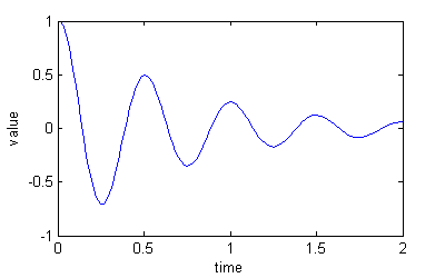
Here’s a graph showing  and
and  (2Hz). You can see that the oscillation magnitude is reduced by 50% every half second, i.e. 25% every second.
Conclusion
I’ve discussed how to implement numeric springing using the faster but less stable semi-implicit Euler method, the difference between numeric springing versus tweening, and the half-life parameterization of numeric springing.
I hope this post has given you a better understanding of various aspects and applications of numeric springing.