Game Math: Dot Product, Rulers, And Bouncing Balls

Source files and future updates are available on Patreon.
You can follow me on Twitter.

This post is part of my Game Math Series.

本文之中文翻譯在此

Prerequisites

Overview

The dot product is a simple yet extremely useful mathematical tool. It encodes the relationship between two vectors’ magnitudes and directions into a single value. It is useful for computing projection, reflection, lighting, and so much more.

In this tutorial, you’ll learn:

The geometric meaning of the dot product.
How to project one vector onto another.
How to measure an object’s dimension along an arbitrary ruler axis.

How to reflect a vector relative to a plane.
How to bounce a ball off a slope.

The Dot Product

Let’s say we have two vectors, $\vec{a}$ and $\vec{b}$ . Since a vector consists of just a direction and a magnitude (length), it doesn’t matter where we place it in a figure. Let’s position $\vec{a}$ and $\vec{b}$ so that they start at the same point:

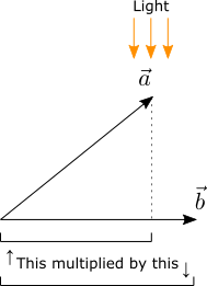
The dot product is a mathematical operation that takes two vectors as input and returns a scalar value as output. It is the product of the signed magnitude of the first vector’s projection onto the second vector and the magnitude of the second vector. Think of projection as casting shadows using parallel light in the direction perpendicular to the vector being projected onto:

We write the dot product of $\vec{a}$ and $\vec{b}$ as $\vec{a} \cdot \vec{b}$ (read a dot b).

If the angle between the two vectors is less than 90 degrees , the signed magnitude of the first vector is positive (thus simply the magnitude of the first vector). If the angle is larger than 90 degrees, the signed magnitude of the first vector is its negated magnitude.

Which one of the vectors is “the first vector” doesn’t matter. Reversing the vector order gives the same result:

$\begin{flalign*} \vec{a} \cdot \vec{b} = \vec{b} \cdot \vec{a} \end{flalign*}$

If $\vec{b}$ is a unit vector, the signed magnitude of the projection of $\vec{a}$ onto $\vec{b}$ is simply $\vec{a} \cdot \vec{b}$ .

Cosine-Based Dot Product Formula

Notice that there’s a right triangle in the figure. Let the angle between $\vec{a}$ and $\vec{b}$ be $\theta$ :

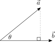
Recall from this tutorial that the length of the adjacent side of a right triangle is the length of its hypotenuse multiplied by the cosine of the angle $\theta$ , so the signed magnitude of the projection of $\vec{a}$ onto $\vec{b}$ is $\lvert \vec{a} \rvert \cos{\theta}$ :

So the dot product of two vectors can be expressed as the product of each vector’s magnitude and the cosine of the angle between the two, which also reaffirms the property that the order of the vectors doesn’t matter:

$\begin{flalign*} \vec{a} \cdot \vec{b} = \lvert \vec{a} \rvert \lvert \vec{b} \rvert \cos{\theta} \end{flalign*}$

If both $\vec{a}$ and $\vec{b}$ are unit vectors, then $\vec{a} \cdot \vec{b}$ simply equals to $\cos{\theta}$ .

If the two vectors are perpendicular (angle in between is $90^\circ$ ), the dot product is zero. If the angle between the two vectors is smaller than $90^\circ$ , the dot product is positive. If the angle is larger than $90^\circ$ , the dot product is negative. Thus, we can use the sign of the dot product of two vectors to get a very rough sense of how aligned their directions are.

Since $\cos{0^\circ} = 1$ monotonically decreases all the way to $\cos{180^\circ} = -1$ , the more similar the directions of the two vectors are, the larger their dot product; the more opposite the directions of the two vectors are, the smaller their dot product. In the extreme cases where the two vectors point in the exact same direction ( $\theta = 0$ ) and the exact opposite directions ( $\theta = 180^\circ$ ), their dot products are $\lvert \vec{a} \rvert \lvert \vec{b} \rvert$ and $- \lvert \vec{a} \rvert \lvert \vec{b} \rvert$ , respectively.

Component-Based Dot Product Formula

When we have two 3D vectors as triplets of floats, it isn’t immediately clear what the angle in between them are. Luckily, there’s an alternate way to compute the dot product of two vectors that doesn’t involve taking the cosine of the angle in between. Let’s denote the components of $\vec{a}$ and $\vec{b}$ as follows:

$\begin{flalign*} \vec{a} &= (a_x, a_y, a_z) \\ \vec{b} &= (b_x, b_y, b_z) \end{flalign*}$

Then the dot product of the two vectors is also equal to the sum of component-wise products, and can be written as:

$\begin{flalign*} \vec{a} \cdot \vec{b} = a_x b_x + a_y b_y + a_z b_z \end{flalign*}$

Simple, and no cosine needed!

Unity provides a function Vector3.Dot for computing the dot product of two vectors:

float dotProduct = Vector3.Dot(a, b);

Here is an implementation of the function:

Vector3 Dot(Vector3 a, Vector b)
{
  return a.x * b.x + a.y * b.y + a.z * b.z;
}

The formula for computing a vector’s magnitude is $\lvert \vec{a} \rvert = \sqrt{a_x^2 + a_y^2 + a_z^2}$ and can also be expressed using the dot product of the vector with itself:

$\begin{flalign*} \lvert \vec{a} \rvert = \sqrt{\vec{a} \cdot \vec{a}} \end{flalign*}$

Recall the formula $\vec{a} \cdot \vec{b} = \lvert \vec{a} \rvert \lvert \vec{b} \rvert \cos{\theta}$ . This means if we know the dot product and the magnitudes of two vectors, we can reverse-calculate the angle between them by using the arccosine function:

$\begin{flalign*} \theta = \cos^{-1}{(\frac{\vec{a} \cdot \vec{b}}{\lvert \vec{a} \rvert \lvert \vec{b} \rvert})} \end{flalign*}$

If $\vec{a}$ and $\vec{b}$ are unit vectors, we can further simplify the formulas above by skipping the computation of vector magnitudes:

$\begin{flalign*} \vec{a} \cdot \vec{b} &= \cos{\theta} \\ \theta &= \cos^{-1}{(\vec{a} \cdot \vec{b})} \end{flalign*}$

Vector Projection

Now that we know the geometric meaning of the dot product as the product of a projected vector’s signed magnitude and another vector’s magnitude, let’s see how we can project one vector onto another. Let $\vec{c} = {project}_{\vec{b}}(\vec{a})$ denote the projection of $\vec{a}$ onto $\vec{b}$ :

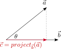
The unit vector in the direction of $\vec{b}$ is $\frac{\vec{b}}{\lvert \vec{b} \rvert}$ , so if we scale it by the signed magnitude of the projection of $\vec{a}$ onto $\vec{b}$ , then we will get $\vec{c}$ . In other words, $\vec{c}$ is parallel to the direction of $\vec{b}$ and has a magnitude equal to that of the projection of $\vec{a}$ onto $\vec{b}$ .

Since the dot product $\vec{a} \cdot \vec{b}$ is the product of the magnitude of $\vec{b}$ and the signed magnitude of the projection of $\vec{a}$ onto $\vec{b}$ , the signed magnitude of $\vec{c}$ is just the dot product of $\vec{a}$ and $\vec{b}$ divided by the magnitude of $\vec{b}$ :

$\begin{flalign*} \frac{\vec{a} \cdot \vec{b}}{\lvert \vec{b} \rvert} \end{flalign*}$

Multiplying this signed magnitude with the unit vector $\frac{\vec{b}}{\lvert \vec{b} \rvert}$ gives us the formula for vector projection:

$\begin{flalign*} \vec{c} = {project}_{\vec{b}}(\vec{a}) = \frac{\vec{a} \cdot \vec{b}}{{\lvert \vec{b} \rvert}^2} \: \vec{b} \end{flalign*}$

Recall that ${\lvert \vec{b} \rvert}^2 = \vec{b} \cdot \vec{b}$ , so we can also write the projection formula as:

$\begin{flalign*} {project}_{\vec{b}}(\vec{a}) = \frac{\vec{a} \cdot \vec{b}}{\vec{b} \cdot \vec{b}} \: \vec{b} \end{flalign*}$

And if $\vec{b}$ , the vector to project $\vec{a}$ onto, is a unit vector, the projection formula can be further simplified:

$\begin{flalign*} {project}_{\vec{b}}(\vec{a}) = (\vec{a} \cdot \vec{b}) \: \vec{b} \end{flalign*}$

Unity provides a function Vector3.Project that computes the projection of one vector onto another:

Vector3 projection = Vector3.Project(vec, onto);

Here is an implementation of the function:

Vector3 Project(Vector3 vec, Vector3 onto)
{
  float numerator = Vector3.Dot(vec, onto);
  float denominator = Vector3.Dot(onto, onto);
  return (numerator / denominator) * onto;
}

Sometimes we need to guard against a potential degenerate case, where the vector being projected onto is a zero vector or a vector with an overly small magnitude, producing a numerical explosion as the projection involves division by zero or near-zero. This can happen with Unity’s Vector3.Project function.

One way to handle this is to compute the magnitude of the vector being projected onto. Then, if the magnitude is too small, use a fallback vector (e.g. the unit +X vector, the forward vector of a character, etc.):

Vector3 SafeProject(Vector3 vec, Vector3 onto, Vector3 fallback)
{
  float sqrMag = v.sqrMagnitude;
  
  if (sqrMag &gt; Epsilon) // test against a small number
    return Vector3.Project(vec, onto);
  else
    return Vector3.Project(vec, fallback);
}

Exercise: Ruler

Here’s an exercise for vector projection: make a ruler that measures an object’s dimension along an arbitrary axis.

A ruler is represented by a base position (a point) and an axis (a unit vector):

struct Ruler
{
  Vector3 Base;
  Vector3 Axis;
}

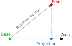
Here’s how you project a point onto the ruler. First, find the relative vector from the ruler’s base position to the point. Next, project this relative vector onto the ruler’s axis. Finally, the point’s projection is the ruler’s base position offset by the projected relative vector:

Vector3 Project(Vector3 vec, Ruler ruler)
{
  // compute relative vector
  Vector3 relative = vec - ruler.Base;
  
  // projection
  float relativeDot = Vector3.Dot(vec, ruler.Axis);
  Vector3 projectedRelative = relativeDot * ruler.Axis;

  // offset from base
  Vector3 result = ruler.Base+ projectedRelative;

  return result;
}

The intermediate relativeDot value above basically measures how far away the point’s projection is from the ruler’s base position, in the direction of the ruler’s axis if positive, or in the opposite direction of the ruler’s axis if negative.

If we compute such measurement for each vertex of an object’s mesh and find the minimum and maximum measurements, then we can obtain the object’s dimension measured along the ruler’s axis by subtracting the minimum from the maximum. Offsetting from the ruler’s base position by the ruler’s axis vector multiplied by these two extreme values gives us the two ends of the projection of the object onto the ruler.

void Measure
(
  Mesh mesh, 
  Ruler ruler, 
  out float dimension, 
  out Vector3 minPoint, 
  out Vector3 maxPoint
)
{
  float min = float.MaxValue;
  float max = float.MinValue;

  foreach (Vector3 vert in mesh.vertices)
  {
    Vector3 relative = vert- ruler.Base;
    float relativeDot = Vector3.Dot(relative , ruler.Axis);
    min = Mathf.Min(min, relativeDot);
    max = Mathf.Max(max, relativeDot);
  }
  
  dimension = max - min;
  minPoint = ruler.Base+ min * ruler.Axis;
  maxPoint = ruler.Base+ max * ruler.Axis;
}

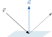
Vector Reflection

Now we are going to take a look at how to reflect a vector, denoted $\vec{v}$ , relative to a plane with its normal vector denoted $\vec{n}$ :

We can decompose the vector to be reflected into a parallel component (denoted $\vec{v}_\parallel$ ) and a perpendicular component (denoted $\vec{v}_\perp$ ) with respect to the plane:

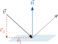
$\begin{flalign*} \vec{v} = \vec{v}_\parallel + \vec{v}_\perp \end{flalign*}$

The perpendicular component is the projection of the vector onto the plane’s normal, and the parallel component can be obtained by subtracting the perpendicular component from the vector:

$\begin{flalign*} \vec{v}_\perp &= {project}_{\vec{n}}(\vec{v}) \\ \vec{v}_\parallel &= \vec{v} - \vec{v}_\perp \end{flalign*}$

Flipping the direction of the perpendicular component and adding it to the parallel component gives us the reflected vector off the plane.

Let’s denote the reflection ${reflect}_\vec{n}}(\vec{v}$ ):

$\begin{flalign*} {reflect}_{\vec{n}}(\vec{v}) = \vec{v}_\parallel - \vec{v}_\perp \end{flalign*}$

If we substitute $\vec{v}_\parallel$ with $\vec{v} - \vec{v}_\perp$ , we get an alternative formula:

$\begin{flalign*} {reflect}_{\vec{n}}(\vec{v}) = \vec{v} - 2\vec{v}_\perp \end{flalign*}$

Unity provides a function Vector3.Reflect for computing vector reflection:

float reflection = Vector3.Reflect(vec, normal);

Here is an implementation of the function using the first reflection formula:

Vector3 Reflect(Vector vec, Vector normal)
{
  Vector3 perpendicular= Vector3.Project(vec, normal);
  Vector3 parallel = vec - perpendicular;
  return parallel - perpendicular;
}

And here is an implementation using the alternative formula:

Vector3 Reflect(Vector vec, Vector normal)
{
  return vec - 2.0f * Vector3.Project(vec, normal);
}

Exercise: Bouncing A Ball Off A Slope

Now that we know how to reflect a vector relative to a plane, we are well-equipped to simulate a ball bouncing off a slope.

We are going to use the Euler Method mentioned in a previous tutorial to simulate the trajectory of a ball under the influence of gravity.

ballVelocity+= gravity * deltaTime;
ballCenter += ballVelocity* deltaTime;

In order to detect when the ball hits the slope, we need to know how to detect when a ball penetrates a plane.

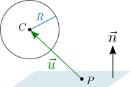
A sphere can be defined by a center and a radius. A plane can be defined by a normal vector and a point on the plane. Let’s denote the sphere’s center $C$ , the sphere radius $R$ , the plane normal $\vec{n}$ (a unit vector), and a point on the plane $P$ . Also, let the vector from $P$ to $C$ be denoted $\vec{u}$ .

If the sphere does not penetrate the plane, the component of $\vec{u}$ perpendicular to the plane, denoted $\vec{u}_\perp$ , should be in the same direction as $\vec{n}$ and have a magnitude no less than $R$ .

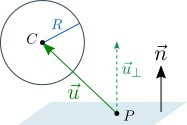
In other words, the sphere does not penetrate the plane if $\vec{u} \cdot \vec{n} > R$ ; otherwise, the sphere is penetrating the plane by the amount $R - \vec{u} \cdot \vec{n}$ and its position needs to be corrected.

In order to correct a penetrating sphere’s position, we can simply move the sphere in the direction of the plane’s normal $\vec{n}$ by the penetration amount. This is an approximated solution and not physically correct, but it’s good enough for this exercise.

// returns original sphere center if not penetrating
// or corrected sphere center if penetrating
void SphereVsPlane
(
  Vector3 c,        // sphere center
  float r,          // sphere radius
  Vector3 n,        // plane normal (unit vector)
  Vector3 p,        // point on plane
  out Vector3 cNew, // sphere center output
)
{
  // original sphere position as default result
  cNew = c;

  Vector3 u = c - p;
  float d = Vector3.Dot(u, n);
  float penetration = r - d;

  // penetrating?
  if (penetration &gt; 0.0f)
  {
    cNew = c + penetration * n;
  }
}

And then we insert the positional correction logic after the integration.

ballVelocity += gravity * deltaTime;
ballCenter += ballVelocity* deltaTime;

Vector3 newSpherePosition;
SphereVsPlane
(
  ballCenter, 
  ballRadius, 
  planeNormal, 
  pointOnPlane, 
  out newBallPosition
);

ballPosition = newBallPosition;

We also need to reflect the sphere’s velocity relative to the slope upon positional correction due to penetration, so it bounces off correctly.

The animation above shows a perfect reflection and doesn’t seem natural. We’d normally expect some sort of degradation in the bounced ball’s velocity, so it bounces less with each bounce.

This is typically modeled as a restitution value between the two colliding objects. With 100% restitution, the ball would bounce off the slope with perfect velocity reflection. With 50% restitution, the magnitude of the ball’s velocity component perpendicular to the slope would be cut in half. The restitution value is the ratio of magnitudes of the ball’s perpendicular velocity components after versus before the bounce. Here is a revised vector reflection function with restitution taken into account:

Vector3 Reflect
(
  Vector3 vec, 
  Vector3 normal, 
  float restitution
)
{
  Vector3 perpendicular= Vector3.Project(vec, normal);
  Vector3 parallel = vec - perpendicular;
  return parallel - restitution * perpendicular;
}

Here is the modified SphereVsPlane function that takes variable restitution into account:

// returns original sphere center if not penetrating
// or corrected sphere center if penetrating
void SphereVsPlane
(
  Vector3 c,        // sphere center
  float r,          // sphere radius
  Vector3 v,        // sphere velocity
  Vector3 n,        // plane normal (unit vector)
  Vector3 p,        // point on plane
  float e,          // restitution
  out Vector3 cNew, // sphere center output
  out Vector3 vNew  // sphere velocity output
)
{
  // original sphere position &amp; velocity as default result
  cNew = c;
  vNew = v;

  Vector3 u = c - p;
  float d = Vector3.Dot(u, n);
  float penetration = r - d;

  // penetrating?
  if (penetration &gt; 0.0f)
  {
    cNew = c + penetration * n;
    vNew = Reflect(v, n, e);
  }
}

And the positional correction logic is replaced with a complete bounce logic:

ballVelocity+= gravity * deltaTime;
spherePosition += ballVelocity* deltaTime;

Vector3 newSpherePosition;
Vector3 newSphereVelocity;
SphereVsPlane
(
  spherePosition , 
  ballRadius, 
  ballVelocity, 
  planeNormal, 
  pointOnPlane, 
  restitution, 
  out newBallPosition, 
  out newBallVelocity;
);

ballPosition= newBallPosition;
ballVelocity= newBallVelocity;

Finally, now we can have balls with different restitution values against a slope:

Summary

In this tutorial, we have been introduced to the geometric meaning of the dot product and its formulas (cosine-based and component-based).

We have also seen how to use the dot product to project vectors, and how to use vector projection to measure objects along an arbitrary ruler axis.

Finally, we have learned how to use the dot product to reflect vectors, and how to use vector reflection to simulate balls bouncing off a slope.

If you enjoyed this tutorial and would like to see more, please consider supporting me on Patreon. By doing so, you can also get updates on future tutorials. Thanks!

2 Responses to Game Math: Dot Product, Rulers, And Bouncing Balls

behram says:

January 24, 2020 at 03:32

This is very a well tutorial !
The small exercises to reinforce the concepts are a big win.

Consider doing something like this on Udemy.

Cheers
b

Josh says:

January 19, 2020 at 08:24

This is a great tutorial. Thanks!

Prerequisites

Overview

The Dot Product

Cosine-Based Dot Product Formula

Component-Based Dot Product Formula

Vector Projection

Exercise: Ruler

Vector Reflection

Exercise: Bouncing A Ball Off A Slope

Summary

Related

About Allen Chou

2 Responses to Game Math: Dot Product, Rulers, And Bouncing Balls

Leave a Reply Cancel reply

Search

Follow Me

Categories

Archives

Meta

Feeds

Game Math: Dot Product, Rulers, And Bouncing Balls

Prerequisites

Overview

The Dot Product

Cosine-Based Dot Product Formula

Component-Based Dot Product Formula

Vector Projection

Exercise: Ruler

Vector Reflection

Exercise: Bouncing A Ball Off A Slope

Summary

Share this:

Related

About Allen Chou

2 Responses to Game Math: Dot Product, Rulers, And Bouncing Balls

Leave a Reply Cancel reply

Search

Follow Me

Categories

Archives

Meta

Feeds