Game Math: Trigonometry Basics – Tangent, Triangles, And Cannonballs | Ming-Lun "Allen" Chou

Source files and future updates are available on Patreon.
You can follow me on Twitter.

This post is part of my Game Math Series.

本文之中文翻譯在此

Prerequisite

Trignometry Basics – Sine & Cosine

Overview

In the previous tutorial, we have learned about two basic trigonometric functions: sine & cosine. This time, we are going to look at another basic trigonometric function: tangent. Together, these three functions form the basis of trigonometry, and they can be used to solve all sorts of geometric problems that arise in game development.

In this tutorial, you’ll learn:

A geometric interpretation of another basic trigonometric function: tangent.
The relationships among sine, cosine, and tangent.
How to use tangent to create smooth intro and outro motion.

How to relate angles and sides of right triangles using trigonometric functions.
How to simulate a cannonball, given an initial speed and an elevation angle.
How to draw predicted trajectories even before firing the cannonball.

How to place cannonball targets, given a horizontal distance and an elevation angle.

Geometric Interpretation of Tangent

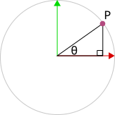
Let’s look at the unit circle from the last tutorial, with a point $P$ on it, as well as the angle $\theta$ between the X axis (+X direction) and the line segment formed by $P$ and the origin.

Recall that the coordinates $(X, Y)$ of $P$ is $(\cos\theta, \sin\theta)$ . This time we are going to look at a new trigonometric function: $\tan\theta$ (tangent of theta). It is the slope of the line segment between $P$ and the origin.

The slope of a line is its ratio of vertical change versus horizontal change. For example, let’s look at this line segment:

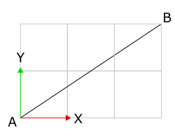
To move from point $A$ to point $B$ , we walk 3 units in the +X direction and then 2 units in the +Y direction, so the slop of the line is $\frac{2}{3}$ .

And for a line segment that goes “downhill” like this:

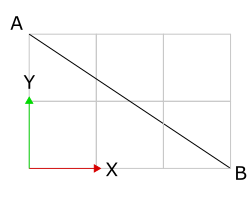
The slope would be $\frac{-2}{3}$ , a negative value, since the vertical change versus horizontal change is negative.

Now, back to the unit circle figure:

We see that moving from the origin to $P$ involves a horizontal change of $\cos\theta$ and a vertical change of $\sin\theta$ , so the slope of the line segment between the origin and $P$ is $\frac{\sin\theta}{\cos\theta}$ , hence $\tan\theta = \frac{\sin\theta}{\cos\theta}$ .

But that’s just a mathematical expression. Here’s where $\tan\theta$ visually fits into the unit circle figure. Let’s draw a tangential line to the circle at $P$ , i.e. a line that goes through $P$ and is perpendicular to the line segment between $P$ and the origin:

Let’s just look at the portion of this tangential line that is between $P$ and the X axis, and mark up some of the points:

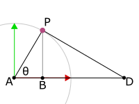
The angles $\angle ABP$ and $\angle APD$ are right angles. And $\angle PAB = \angle PAD = \theta$ . Let $\overline{AB}$ denote the length of the line segment between point $A$ and point $B$ .

Now, split the figure into two triangles:

Since all internal angles of a triangle add up to $180^\circ$ and both triangles have an angle of $\theta$ and $90^\circ$ , the unmarked angles from both triangles, $\angle APB$ and $\angle ADP$ , are exactly the same: $180^\circ - \theta - 90^\circ$ .

If two triangles have identical sets of angles, then they are similar, i.e. if you proportionally scale, rotate, and/or flip one of them, it can become identical to the other one.

When two triangles are similar, the ratio between the lengths of two sides from one triangle equals to the ratio between the lengths of the corresponding sides of the other triangle. Thus:

$\begin{flalign*} \frac{\overline{BP}}{\overline{AB}} = \frac{\overline{DP}}{\overline{AP}} \end{flalign*}$

We know that the coordinates of $P$ are $(\cos\theta, \sin\theta)$ , so $\overline{AB} = \cos\theta$ and $\overline{BP} = \sin\theta$ . And we know that $\overline{AP}$ is equal to the radius of the unit circle, so $\overline{AP}=1$ . Now the equation above becomes:

$\begin{flalign*} \frac{\sin\theta}{\cos\theta} = \frac{\overline{DP}}{1} \end{flalign*}$

And we know that $\tan\theta = \frac{\sin\theta}{\cos\theta}$ , so we get:

$\begin{flalign*} \tan\theta = \overline{DP} \end{flalign*}$

We have found the visual representation of $\tan\theta$ !

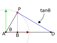
The absolute value of $\tan\theta$ is the length of the portion of the tangential line between point $P$ and the X axis. Notice that I said absolute value, because depending on the signs of $\sin\theta$ and $\cos\theta$ , $\tan\theta$ can be positive or negative. This animation highlights (in blue) the line segment whose length is equal to the absolute value of $\tan\theta$ :

The Tangent Curve

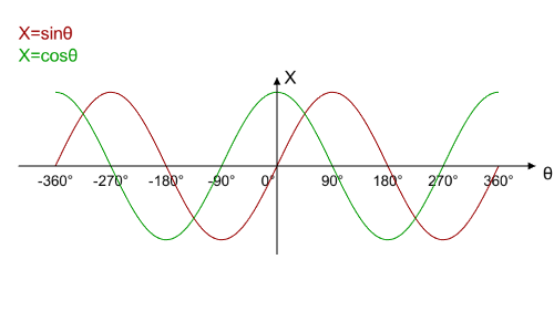
We’ve seen the plots for $\sin\theta$ and $\cos\theta$ versus $\theta$ in the previous tutorial. Let’s overlay them on top of each other:

And now let’s add $\tan\theta$ into the mix:

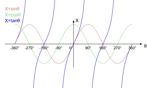
Notice how, unlike $\sin\theta$ and $\cos\theta$ , the value of $\tan\theta$ is not constrained within the $[-1, 1]$ range. Since $\tan = \frac{\sin\theta}{\cos\theta}$ , the absolute value of $\tan\theta$ approaches infinity as $\cos\theta$ approaches zero. Also, unlike $\sin\theta$ and $\cos\theta$ , the period of $\tan\theta$ is $\pi$ , instead of $2\pi$ .

Another thing worth noting is the relationships among the signs of the three basic trigonometric functions. Since $\tan\theta = \frac{\sin\theta}{\cos\theta}$ , the sign of $\tan\theta$ is positive when $\sin\theta$ and $\cos\theta$ have the same sign, and is negative otherwise.

Now, let’s try plugging the tangent curve over time into the X coordinate of an object:

float tan = Mathf.Tan(Rate * Time.time);
obj.transform.position = Vector3(tan, 0.0f, 0.0f);

The object comes in fast from the $-X$ direction, slows down a bit, and then runs off fast again towards the $+X$ direction.

We can utilize this motion to create effects like these falling stars:

float tan = Mathf.Tan(Rate * Time.time);
obj.transform.position = center + moveDirection * tan;

The acceleration and deceleration are kind of subtle. We can further amplify the effect by raising the tangent function to a power of, say, 3:

float tan = Mathf.Tan(Rate * Time.time);
float tan3 = tan * tan * tan;
obj.transform.position = center + moveDirection * tan3;

Trigonometric Functions, Angles, And Triangles

So we’ve seen how the three basic trigonometric functions relate to the unit circle. Now we’re going to take a look at their relationships with triangles. They are called trigonometric functions, after all. Specifically, we’re going to look at right triangles (triangles with a right angle).

First, let’s get the terminologies out of the way. Here is a right triangle with an angle marked up as $\theta$ :

The side of the triangle between $\theta$ and the right angle is called the adjacent side, since it is adjacent to $\theta$ . The other side next to the right angle is called the opposite side, because it is across from $\theta$ . The remaining (also the longest) side opposed to the right angle is called the hypotenuse:

And here is how the three basic trigonometric functions relate to the lengths of the triangle sides:

$\sin\theta=$ length of the opposite side divided by length of the hypotenuse.
$\cos\theta=$ length of the adjacent side divided by length of the hypotenuse.
$\tan\theta=$ length of the opposite side divided by length of the adjacent side.

Or, in mathematical form:

$\begin{alignat*} \ \sin\theta &= \frac{opposite}{hypotenuse} \:\:\: \ \cos\theta &= \frac{adjacent}{hypotenuse} \:\:\: \ \tan\theta &= \frac{opposite}{adjacent} \end{alignat*}$

These equations could be a bit too much to remember. Here’s a common verbal mnemonic that might help: soh-cah-toa (sine is the opposite side divided by the hypotenuse, cosine is the adjacent side divided by the hypotenuse, and tangent is the opposite side divided by the adjacent side).

I did not learn this verbal mnemonic in Taiwan (my math classes were taught in Mandarin). What I learned was a visual mnemonic that I’m quite fond of: Write the initials of sine, cosine, and tangent in cursive, along with the right triangle as shown below (please forgive my ugly handwriting).

When you write an initial, the corresponding function equals the length of the first side you write past dividing the length of the second side you write past:

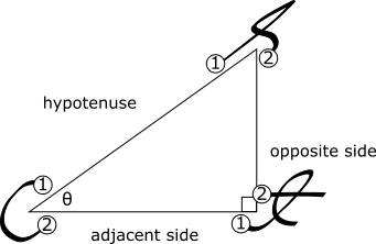
$\sin\theta=$ length of the hypotenuse dividing length of the opposite side.
$\cos\theta=$ length of the hypotenuse dividing length of the adjacent side.
$\tan\theta=$ length of the adjacent side dividing length of the opposite side.

When describing fractions in Mandarin, instead of saying “A divided by B”, we say “B dividing A”. That’s why this mnemonic orders the divisor before the dividend in its wording. This ordering might not be intuitive to native English speakers, but if you find it useful, then great!

Now back to the equations:

$\begin{alignat*} \ \sin\theta &= \frac{opposite}{hypotenuse} \:\:\: \ \cos\theta &= \frac{adjacent}{hypotenuse} \:\:\: \ \tan\theta &= \frac{opposite}{adjacent} \end{alignat*}$

Whatever the size of the right triangle, the equations above always hold true, because ratios between two sides are independent of the absolute lengths of individual sides.

If we scale the triangle so that the hypotenuse is of length 1, then we can fit it back into our unit circle figure, with $(X, Y)$ being the coordinates of point $P$ on the circle:

And the equations above agree nicely with the coordinates of $P$ , $(X, Y) = (\cos\theta, \sin\theta)$ :

$\begin{alignat*} \ \sin\theta &= \frac{Y}{1} &&= Y \:\:\:\: \ \cos\theta &= \frac{X}{1} &&= X \:\:\:\: \ \tan\theta &= \frac{Y}{X} &&= \frac{\sin\theta}{\cos\theta} \end{alignat*}$

Knowing the equations for trigonometric functions in terms of lengths of right triangle sides, for any given right triangle with an angle $\theta$ , if we know the length of any one side, we can derive the lengths of the other two sides using the three basic trigonometric functions.

Let $J$ denote the length of the adjacent side, $S$ the length of the opposite side, and $H$ the length of the hypotenuse:

If we know the length of the hypotenuse ( $H$ ), then $J = H \cos\theta$ , and $S = H \sin\theta$ :

If we know the length of the adjacent side ( $J$ ), then $S = J \tan\theta$ , and $H = \frac{J}{\cos\theta}$ :

If we know the length of the opposite side ( $S$ ), then $J = \frac{S}{\tan\theta}$ , and $H = \frac{S}{\sin\theta}$ :

Simulating Cannonballs & Predicting Trajectories

Finally, it’s time for practical examples! Let’s see how we can simulate cannonballs when given an initial speed, a horizontal angle, and an elevation angle. Also, let’s find out how we can display the predicted trajectories even before firing the cannon.

But before all that, here’s a very quick recap on some basic terminologies in motion dynamics. An object’s position is where the object is physically located. An object’s velocity is the rate of change in its position (typically expressed as change of position per second). An object’s acceleration is the rate of change in its velocity (typically expressed as change of velocity per second).

The Euler Method is a quick and easy algorithm for simulating object movement: For each moving object, we store its velocity vector along with its position. For each update, or time step, we change the velocity by acceleration times delta time (the time difference between each update), and then we change the position by velocity times delta time:

velocity += acceleration * deltaTime;
position += velocity * deltaTime;

To simulate gravity at ground level and at human scale, we let the acceleration be a constant downward-pointing vector. Here’s an example of how an object would move in 2D under the influence of gravity when starting off with an initial velocity pointing up and to the right, simulated using the Euler Method:

If we simulate the entire trajectory within a single frame by performing multiple time steps, and draw a little dot once every several iterations, we can get ourselves a nice indicator of the predicted trajectory:

velocity = initialVelocity;
position = initialPosition;
for (int i = 0; i &lt; NumIterations; ++i)
{
  velocity += acceleration * deltaTime;
  position += velocity * deltaTime;
  
  if (i % IterationsPerDot != 0)
    continue;
  
  DrawDot(position);
}

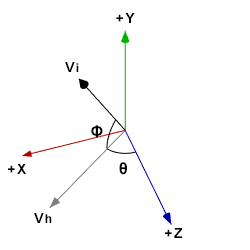
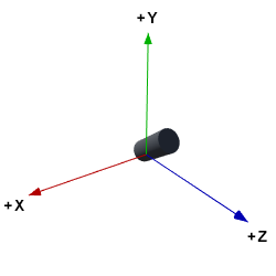
Now, let’s compute the initial velocity of a cannonball if it is fired from the cannon at an initial speed $K$ (length of the initial velocity vector), a horizontal angle $\theta$ , and an elevation angle $\phi$ (phi). Let the $+Z$ direction be the cannon’s forward direction and the $+X$ direction be its right direction (Unity uses left-hand coordinates).

To compute the initial velocity, we need to first compute a unit vector (vector of length 1) in the same direction. Once we have that unit vector, we can simply multiply all its components by a the desired speed $K$ to obtain the initial velocity vector.

The diagram below shows the a unit vector in the $+X$ direction in red, a unit vector in the $+Y$ direction in green, a unit vector in the $+Z$ direction in blue, a unit vector in the direction of initial velocity in black (labeled $V_i$ ), a unit vector in the horizontal direction of the initial velocity in gray (labeled $V_h$ ), the horizontal angle $\theta$ (between $+Z$ and $V_h$ ), and the elevation angle $\phi$ (between $V_h$ and $V_i$ ):

The goal is to find $V_i$ and multiply it with $K$ . We can isolate the unit vectors and angles from the diagram above into two unit circle diagrams.

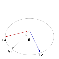
One is a horizontal unit circle diagram with $+X$ , $+Z$ , $V_h$ , and $\theta$ :

And the other one is a vertical unit circle diagram with $+Y$ , $V_h$ , $V_i$ , and $\phi$ :

If we view the first (horizontal) unit circle diagram from a different angle, we’ll get a familiar view of a flat unit circle:

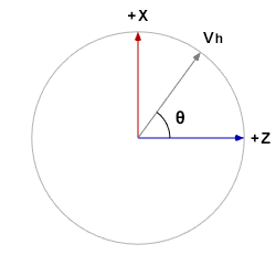
We’ve done this math before. The component of $V_h$ in the drection of $+Z$ is of length $\cos\theta$ , and the component in the direction of $+X$ is of length $\sin\theta$ . This gives us $V_h = (\sin\theta, 0, \cos\theta)$ .

Now, view the second (vertical) unit circle diagram from a different angle that gives us the same familiar view of a flat unit circle:

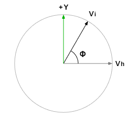
It’s the same drill. The component of $V_i$ in the direction of $V_h$ is of length $\cos\phi$ , and the component in the direction of $+Y$ is of length $\sin\phi$ , so we can now compute $V_i$ :

$\begin{flalign*} V_i &= \cos\phi \cdot V_h + \sin\phi \cdot (0, 1, 0) \\ &= (\cos\phi \sin\theta, \: \sin\phi, \: \cos\phi \cos\theta) \end{flalign*}$

Multiplying $V_i$ with $K$ gives us our initial velocity vector:

$\begin{flalign*} V_i &= K \cdot (\cos\phi \sin\theta, \: \sin\phi, \: \cos\phi \cos\theta) \\ &= (K \cos\phi \sin\theta, \: K \sin\phi, \: K \cos\phi \cos\theta) \end{flalign*}$

And the corresponding code is:

Vector3 ComputeInitialVelocity()
{
  float sinTheta = Mathf.Sin(HorizontalAngle);
  float cosTheta = Mathf.Cos(HorizontalAngle);
  float sinPhi = Mathf.Sin(ElevationAngle);
  float cosPhi = Mathf.Cos(ElevationAngle);

  return
    InitialSpeed
    * new Vector3
      (
        cosPhi * sinTheta, 
        sinPhi, 
        cosPhi * cosTheta
      );
}

Being able to compute the initial velocity vector from a given initial speed, horizontal angle, and elevation angle, we are now well-equipped to simulate a cannonball:

void FireCannon()
{
  velocity = ComputeInitialVelocity();
  obj.transform.position = InitialPosition;
}

void Update()
{
  float dt = Time.deltaTime;
  velocity += acceleration * dt;
  obj.transform.position += velocity * dt;
}

void DrawTrajectory()
{
  float dt = Time.fixedDeltaTime;
  Vector3 velocity = ComputeInitialVelocity();
  Vector3 position = InitialPosition;
  for (int i = 0; i &lt; NumIterations; ++i)
  {
    velocity += acceleration * dt;
    position += velocity * dt;
    
    if (i % IterationsPerDot != 0)
      continue;
    
    DrawDot(position);
}

Placing Cannonball Targets

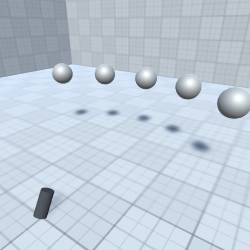
Now that we can fire cannonballs, let’s place some targets. If we want to place a target at a given horizontal distance away from the cannon, as well as at a given elevation angle, where exactly should we place the targets?

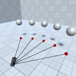
Below is the desired end result. Each target is at a fixed horizontal distance (on the XZ plane) away from the cannon, and is at a fixed elevation angle above ground. The targets are also equally spaced out horizontally, i.e. their horizontal angles relative to the cannon are equally spaced out.

We already know how to compute a horizontal unit vector from a horizontal angle $\theta$ . The horizontal unit vector is $(\cos\theta, 0, \sin\theta)$ . Multiplying such horizontal vector with a given horizontal distance, denoted $D$ , gives us the horizontal offset vector of the target from the cannon: $(D \cos\theta, 0, D \sin\theta)$ . Equally spacing out different $\theta$ and computing the horizontal offset vector for each $\theta$ value gives us the XZ coordinates of the targets (shown as red dots in the image below):

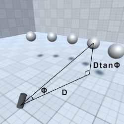
The last step is to determine the Y coordinates of the targets, i.e. how far off ground the targets should be. Recall that if we know the length of the adjacent side to an angle $\theta$ of a right triangle to be $J$ , then the length of the opposite side is $J \tan\theta$ .

Substituting $J$ with the given horizontal distance $D$ and $\theta$ with the elevation angle $\phi$ , the formula for the Y coordinate of the targets becomes $D \tan\phi$ .

We can finally place our targets at the desired positions:

float theta = -0.5f * AngleInterval * (NumTargets - 1);
float elevationTan = Mathf.Tan(ElevationAngle);

foreach (var target in targetArray)
{
  Vector3 horizontalVec = 
    HorizontalDistance 
    * new Vector3
      (
        Mathf.Sin(theta), 
        0.0f, 
        Mathf.Cos(theta)
      );

  theta += AngleInterval;

  Vector3 verticalVec = 
    HorizontalDistance 
    * elevationTan 
    * Vector3.up;

  target.transform.position = 
    Cannon.position 
    + horizontalVec 
    + verticalVec;
}

We haven’t talked about how to detect when a cannonball hits a target or the ground yet. Right now the cannonballs would just go through the targets:

Collision detection is beyond the scope of this tutorial, so I’ll just go over the very basics of sphere-sphere collision really quick.

To detect when a cannonball hits the target, check the distance between the centers of the two and see if it’s less than the sum of their radii. If the cannonball does collide with a target, we destroy the cannonball and the target.

Vector3 cannonballToTargetVec = 
  target.transform.position 
  - cannonball.transform.position;

float cannonballToTargetDist = cannonballToTargetVec.magnitude;
float radiusSum = cannonballRadius + targetRadius;
if (cannonballToTargetDist &lt; radiusSum)
{
  DestroyCannonball();
  DestroyTarget();
}

Using a similar technique when drawing the predicted trajectory, we can terminate the trajectory early when it hits a target.

However, this collision detection technique is discrete, meaning that the cannonball can still go through targets if it travels fast enough. We can mitigate this problem with a continuous collision detection technique, but that is also beyond the scope of this tutorial and will be touched on in later tutorials.

Summary

Previously, we have been introduced to two basic trigonometric functions: sine and cosine. In this tutorial, we have seen a geometric interpretation of another trigonometric function: tangent. We have also learned the relationship among sine, cosine, and tangent, in the context of the unit circle, as well as right triangles.

Next, we have plotted the tangent function alongside sine and cosine; and we are now able to create smooth into and outro motion by utilizing the tangent function.

Finally, using the three basic trigonometric functions, we have learned how to predict and simulate the trajectory of a cannonball, given an initial speed and elevation angle. Plus, we have seen how to place targets, given a horizontal distance and an elevation angle.

We have learned the basics of the three fundamental trigonometric functions that are essential in solving daily gamedev problems. In later tutorials, I will go over more useful mathematical tools that are built on top of these trigonometric functions, as well as some of their practical applications.

If you enjoyed this tutorial and would like to see more, please consider supporting me on Patreon. By doing so, you can also get updates on future tutorials. Thanks!

Game Math: Trigonometry Basics – Tangent, Triangles, And Cannonballs

Prerequisite

Overview

Geometric Interpretation of Tangent

The Tangent Curve

Trigonometric Functions, Angles, And Triangles

Simulating Cannonballs & Predicting Trajectories

Placing Cannonball Targets

Summary

Related

About Allen Chou

Leave a Reply Cancel reply

Search

Follow Me

Categories

Archives

Meta

Feeds

Game Math: Trigonometry Basics – Tangent, Triangles, And Cannonballs

Prerequisite

Overview

Geometric Interpretation of Tangent

The Tangent Curve

Trigonometric Functions, Angles, And Triangles

Simulating Cannonballs & Predicting Trajectories

Placing Cannonball Targets

Summary

Share this:

Related

About Allen Chou

Leave a Reply Cancel reply

Search

Follow Me

Categories

Archives

Meta

Feeds