Game Math: “Projecting” a Curve onto Another

This post is part of my Game Math Series.

Also, this post is part 1 of a series (part 2) leading up to a geometric interpretation of Fourier transform and spherical harmonics.

Fourier transform and spherical harmonics are mathematical tools that can be used to represent a function as a combination of periodic functions (functions that repeat themselves, like sine waves) of different frequencies. You can approximate a complex function by using a limited number of periodic functions at certain frequencies. Fourier transform is often used in audio processing to post-process signals as combination of sine waves of different frequencies, instead of single streams of sound waves. Spherical harmonics can be used to approximate baked ambient lights in game levels.

We’ll revisit these tools in later posts, so it’s okay if you’re still not clear how they can be of use at this point. First, let’s start somewhere more basic.

Projecting a Vector onto Another

If you have two vectors $\vec{a}$ and $\vec{b}$ , projecting $\vec{a}$ onto $\vec{b}$ means stripping out part of $\vec{a}$ that is orthogonal to $\vec{b}$ , so the result is the part of $\vec{a}$ that is parallel to $\vec{b}$ . Here is a figure I borrowed from Wikipedia:

vector projection

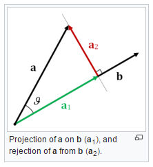
The dot product of $\vec{a}$ and $\vec{b}$ is a scalar equal to the product of magnitude of both vectors and the cosine of the angle ( $\theta$ , using the figure above) between the vectors:

$\vec{a} \cdot \vec{b} = |\vec{a}| |\vec{b}| cos\theta$

Another way of calculating the dot product is adding together the component-wise products. If $\vec{a} = (a_x, a_y, a_z)$ and $\vec{b} = (b_x, b_y, b_z)$ , then:

$\vec{a} \cdot \vec{b} = a_x b_x + a_y b_y + a_z b_z$

A follow-up to the alternate formula above is the formula for vector magnitude. The magnitude of a vector is the square root of the dot product of the vector with itself:

$|\vec{a}| = \sqrt{a_x^2 + a_y^2 + a_z^2} = \sqrt{\vec{a} \cdot \vec{a}}$

The geometric meaning of the dot product $\vec{a} \cdot \vec{b}$ is the magnitude of the projection of $\vec{a}$ onto $\vec{b}$ scaled by $|\vec{b}|$ . Dot product is commutative, i.e. $\vec{a} \cdot \vec{b} = \vec{b} \cdot \vec{a}$ , which means that $\vec{a} \cdot \vec{b}$ is also equal to the magnitude of the projection of $\vec{b}$ onto $\vec{a}$ scaled by $|\vec{a}|$ .

So if you want to get the magnitude of the projection of $\vec{a}$ onto $\vec{b}$ , you need to divide the dot product by the magnitude of $\vec{b}$ :

$|proj(\vec{a}, \vec{b})| = \dfrac{\vec{a} \cdot \vec{b}}{|\vec{b}|} = |\vec{a}| cos\theta$

To get the actual projected vector of $\vec{a}$ onto $\vec{b}$ , multiply the magnitude with the unit vector in the direction of $\vec{b}$ , denoted by $\hat{b}$ :

$proj(\vec{a}, \vec{b}) = (\dfrac{\vec{a} \cdot \vec{b}}{|\vec{b}|}) \hat{b} = (\dfrac{\vec{a} \cdot \vec{b}}{{|\vec{b}|}^2}) \vec{b} = (\dfrac{\vec{a} \cdot \vec{b}}{\vec{b} \cdot \vec{b}}) \vec{b}$

One important property of dot product $\vec{a} \cdot \vec{b}$ is: if it’s positive, the two vectors point in roughly the same direction ( $\theta < 90^\circ$ ); if it’s zero, the vectors are orthogonal ( $\theta = 90^\circ$ ); if it’s negative, the vectors point away from each other ( $\theta > 90^\circ$ ).

For the dot product of two unit vectors, like $\hat{a} \cdot \hat{b}$ , it’s just $cos\theta$ . If it’s 1, then the two vectors point in exactly the same direction ( $\theta = 0^\circ$ ); if it’s -1, then the two vectors point in exactly opposite directions ( $\theta = 180^\circ$ ). So, in order to measure how close the directions two vectors point in, we can normalize both vectors and take their dot product.

Let’s say we have three vectors: $\vec{a}$ , $\vec{b}$ , and $\vec{c}$ . If we want to determine which of $\vec{b}$ and $\vec{c}$ points in a direction closer to where $\vec{a}$ points, we can just compare the dot products of their normalized versions, $\hat{a} \cdot \hat{b}$ and $\hat{a} \cdot \hat{c}$ . Whichever vector’s normalized version has a larger dot product with $\hat{a}$ points in a direction closer to that of $\vec{a}$ .

A metric often used to measure the difference between two data objects is the root mean square error (RMSE) which is the square root of the average of component-wise errors. For vectors, that means:

$RMSE(\vec{a}, \vec{b}) = \sqrt{\frac{1}{3}((a_x - b_x)^2 + (a_y - b_y)^2 + (a_z - b_z)^2)}$

It kind of makes sense, because it is exactly the magnitude of the vector that is the difference between $\vec{a}$ and $\vec{b}$ scaled by $\frac{1}{\sqrt{3}}$ :

$RMSE(\vec{a}, \vec{b}) = (\dfrac{1}{\sqrt{3}})\sqrt{(a_x - b_x)^2 + (a_y - b_y)^2 + (a_z - b_z)^2} = (\dfrac{1}{\sqrt{3}}) |\vec{a} - \vec{b}|$

It’s also the square root of the dot product of the difference vector $\vec{a} - \vec{b}$ with it self scaled by $\frac{1}{\sqrt{3}}$ :

$RMSE(\vec{a}, \vec{b}) = (\dfrac{1}{\sqrt{3}}) |\vec{a} - \vec{b}| = (\dfrac{1}{\sqrt{3}}) \sqrt{(\vec{a} - \vec{b}) \cdot (\vec{a} - \vec{b})}$

Here’s an important property of projection:
The projection of a vector $\vec{a}$ onto another vector $\vec{b}$ is the vector parallel to $\vec{b}$ that has the minimal RMSE with respect to $\vec{a}$ . In other words, $proj(\vec{a}, \vec{b})$ gives you the best scaled version of $\vec{b}$ to approximate $\vec{a}$ .

Also note that if $\hat{a} \cdot \hat{b}$ is larger than $\hat{a} \cdot \hat{c}$ , it means $\hat{b}$ has a smaller RMSE than $\hat{c}$ with respect to $\hat{a}$ ; thus, $\vec{b}$ points in a direction closer to that o $\vec{a}$ than $\vec{c}$ does.

Now we’re finished with vectors. It’s time to move onto curves.

“Projecting” a Curve onto Another

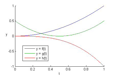
Let’s consider these three curves:

$\begin{flalign*} y &= f(t) = t^2 \\ y &= g(t) = 2(t - \frac{1}{2})^2 \\ y &= h(t) = -t^3 \\ \end{flalign*}$

When working with curves, as opposed to vectors, we need to additionally specify an interval of of interest. For simplicity, we will consider $0 \leq t \leq 1$ for the rest of this post.

Below is a figure showing what they look like side-by-side within our interval of interest:

curves

Just like vectors, “projecting” a curve $f(t)$ onto another curve $g(t)$ gives you the best scaled version of $g(t)$ to approximate $f(t)$ , and the “projection” has minimal RMSE with respect to $f(t)$ . To compute the RMSE of curves, we need to first figure out how to compute the “dot product” of two curves.

Recall that the dot product of vectors is equal to the sum of component-wise products:

$\vec{a} \cdot \vec{b} = a_x b_x + a_y b_y + a_z b_z$

Mirroring that, let’s sum up the products of samples of curves at regular intervals, and we normalize the sum by dividing it with the number of samples, so we don’t get drastically different results due to different number of samples. If we take 10 samples between $0 \leq t \leq 1$ to compute the dot product of $f(t)$ and $g(t)$ , we get:

$f(t) \cdot g(t) = \frac{1}{10} \sum_{i = 1}^{10} f(\frac{i}{10}) g(\frac{i}{10})$

The more samples we use, the more accuracy we get. What if we take an infinite number of samples so we get the most accurate result possible?

$f(t) \cdot g(t) = \lim_{n\to\infty} {\frac{1}{n} \sum_{i = 0}^{n} f(\frac{i}{n}) g(\frac{i}{n}})$

This basically turns into an integral:

$f(t) \cdot g(t) = \int_{0}^{1} f(t) g(t) dt$

So there we have it, one common definition of the “dot product” of two curves:
The integral of the product of two curves over the interval of interest.

Copying the formula from vectors, the RMSE between two curves $f(t)$ and $g(t)$ is:

$RMSE(f(t), g(t)) = \sqrt{(f(t) - g(t)) \cdot (f(t) - g(t))}$

In integral form, it becomes:

$RMSE(f(t), g(t)) = \sqrt{\int_{0}^{1} (f(t) - g(t))^2 dt}$

The “mean” part of the error is omitted since it’s a division by 1, the length of our interval of interest.

To find out which one of the “normalized” version of $g(t)$ and $h(t)$ has less RMSE with respect to the normalized version of $f(t)$ , we take the dot products of the normalized versions of the curves:

$\begin{flalign*} \hat{f}(t) &= \dfrac{f(t)}{|f(t)|} = \dfrac{f(t)}{\sqrt{f(t) \cdot f(t)}} = \sqrt{5}t^2 \\ \hat{g}(t) &= \dfrac{g(t)}{|g(t)|} = \dfrac{g(t)}{\sqrt{g(t) \cdot g(t)}} = 4 \sqrt{5} (t - \dfrac{1}{2})^2 \\ \hat{h}(t) &= \dfrac{h(t)}{|h(t)|} = \dfrac{f(t)}{\sqrt{h(t) \cdot h(t)}} = -\sqrt{7}t^3 \\ \hat{f}(t) \cdot \hat{g}(t) &= \int_{0}^{1} \hat{f}(t) \hat{g}(t) dt = \dfrac{4}{3} \\ \hat{f}(t) \cdot \hat{h}(t) &= \int_{0}^{1} \hat{f}(t) \hat{h}(t) dt = \dfrac{-\sqrt{35}}{6} \\ \end{flalign*}$

The dot product of $\hat{f}(t)$ and $\hat{g}(t)$ is larger than that of $\hat{f}(t)$ and $\hat{h}(t)$ . That means $\hat{g}(t)$ has a lower RMSE than $\hat{h}(t)$ with respect to $\hat{f}(t)$ .

Drawing analogy from vectors, $g(t)$ is conceptually “pointing in a direction” closer to that of $f(t)$ than $h(t)$ does.

Now let’s try finding the best scaled version of $g(t)$ that has minimal RMSE with respect to $f(t)$ , by computing the projection of $f(t)$ onto $g(t)$ :

$proj(f(t), g(t)) = \dfrac{f(t) \cdot g(t)}{g(t) \cdot g(t)} g(t) = \dfrac{4}{3} g(t) = \dfrac{8}{3} (t - \dfrac{1}{2})^2$

And this is what $f(t)$ , $g(t)$ , and $proj(f(t), g(t))$ look like side-by-side:

curve projection

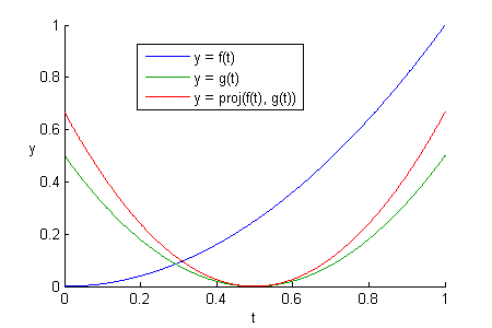
The projected curve $proj(f(t), g(t))$ is a scaled-up version of $g(t)$ that is a better approximation of $f(t)$ than $g(t)$ itself; it is the best scaled version of $g(t)$ that has the least RMSE with respect to $f(t)$ .

Now that you know how to “project” a curve onto another, we will see how to approximate a curve with multiple simpler curves while maintaining minimal error.

1 Response to Game Math: “Projecting” a Curve onto Another

Kamil says:

February 3, 2017 at 02:59

Great article! Applying linear algebra techniques for function was very clever idea. Now I can see how it is really related to the Fourier transform. Can’t wait to see next part 🙂

Projecting a Vector onto Another

“Projecting” a Curve onto Another

Related

About Allen Chou

1 Response to Game Math: “Projecting” a Curve onto Another

Leave a Reply Cancel reply

Search

Follow Me

Categories

Archives

Meta

Feeds

Game Math: “Projecting” a Curve onto Another

Projecting a Vector onto Another

“Projecting” a Curve onto Another

Share this:

Related

About Allen Chou

1 Response to Game Math: “Projecting” a Curve onto Another

Leave a Reply Cancel reply

Search

Follow Me

Categories

Archives

Meta

Feeds